Finding samples
Now it’s time to expose your sample to X-ray photons. Before proceeding, check the status from synoptic to ensure we have a beam on the slit and all valves are open. If the sample rod is still in the UC, ensure that the valve between the Q-chamber and UC is open.
We first start with a 2D spatial map of the sample (a_mp1_x vs. a_mp1_y), after setting a_mp1_yaw at normal incidence. From this point on, you are going to use the control and acquisition software named ‘Scangui’. Here is how we do it:
Mesh scan
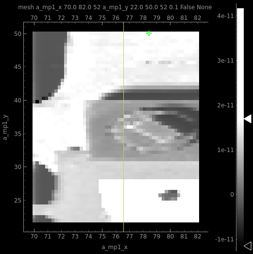
The image above is an example of 2D mapping of a sample plate by FY(fluorescence yield). In the first attempt, the beamline energy does not need to be exactly the resonance energy; rather, any energy a bit higher than the resonant energy will work to get the contrast. You need to open these two softwares: Scangui and Sampletracker
After loading the sample down to the main chamber (we call it the Q-chamber), you first begin with the mesh scan. This is how you can set up the mesh scan in Scangui:
go to ‘MacroExecutor’ or ‘Sequencer’ tab –> find ‘mesh’ macro from the ‘Macro’ dropdown list –> add it –> at the bottom, select the values ‘a_mp1_x’ and ‘a_mp1_y’ under parameters ‘motor1’ and ‘motor2’, respectively –> give start and final motor positions, nr_interval (number of steps), and integ_time. Set bidirectional to ‘true’ or ‘false’.
Linescan
With the Scangui, you can move along x or y while reading an absorption intensity.
From the quickgui: Write down current manipulator positions: a_mp1_x, a_mp1_y, a_mp1_z, and a_mp1_yaw
In the quickgui, choose an appropriate beamline_energy for getting contrast when you are on the sample
In the Scangui, select the measurement group “XAS” (see details on how to change the measurement group in the entry about the Scangui)
In the Scangui, go to basic executor select a_mp1_x or a_mp1_y and scan around your starting guess
In the Scangui, plot a_mp1_x towards the appropriate alba elektrometer signal