Offline Analysis
Data structures
During your experiment the data is recorded in two different .hdf5 files. .hdf5 files are a hierarcichal data structure and behaves much like a “folder”. Each scan or rixs-acquisition has a folder in the files “entry343” or “acq1337”
Scangui/Sardana HDF5 files
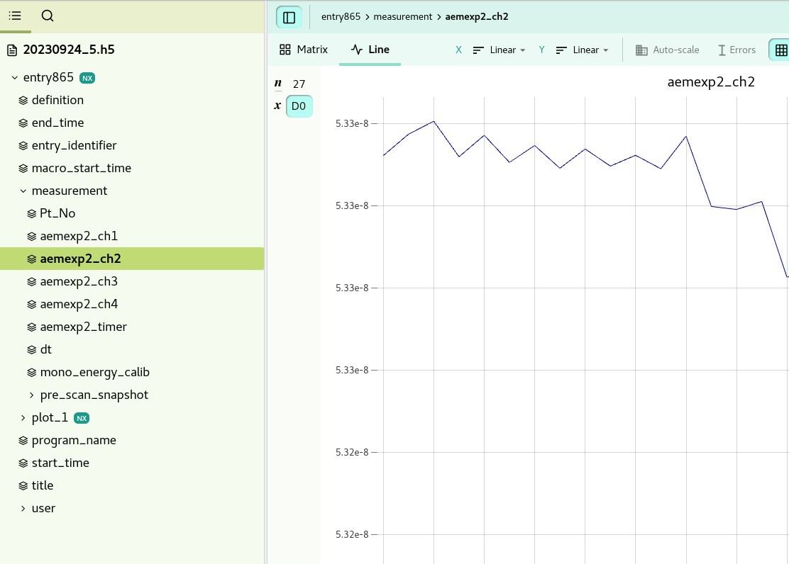
The data recorded for each sardana scan, is selected by the measurement group in the scangui. You will find for example the data from the alba elektrometer in the .hdf5 file under: “entry865/measurement/aemexp2_ch2”.
You can find the start time of the scan under “entry865/start_time”
You find the command that run the scan (with e.g. the beamline range) under “entry865/title”
Before the start of each scan, a pre scan snapshot with some values is recorded. You find e.g. the sample position under “entry865/measurement/pre_scan_snapshot/a_mp1_x”
The hdf5 data can be browsed using https://jupyterhub.maxiv.lu.se/
RIXSaq HDF5 files
Lets use “acq325” as an example. The pre-processed data can be found under: “/acq325/data/calib_x_spectrum” and “/acq325/data/energy_scale”
The raw point-by-point data can be found under: “/acq325/Instrument/DLD8080/data/points” The raw points are 12 columns, each row represent one hit on the detector. The 12 columns are:
x, spatial position, unit in bins 0-8192
y, spatial postion
t, bunch-clock, unit: timebins, the clock is reset to 0 at every revolution of the ring.
t, unixtimestamp, added to the data during readout. Used e.g. for removing the last 5minutes of the measurement.
millisecond counter
start_counter, number of revolutions in the ring. +1 every time the bunch-clock is reset
time_tag, time in 0.5ns bins since a sginal on the time_tag input. Currently connected to one of the manipulator axes.
master_rst_counter, not used
signal1bit, not used
Extra1 (Tango attribute set by the RIXS client, for example the beamline_energy or veritasarm_energy)
Extra2
Extra3
For each scan there is also metadata recorded at the start and the end, you find them in: “/acq325/startmetadata/a_mp1_yaw/position” or “/acq325/endmetadata/a_mp1_yaw/position”
throughout the rixs-measurement, some attributes are also recorded as timestamped data. You can find for example the manipulator position as a function of unixtimestamp here: “/acq325/External/a_mp1_x/position”
The calibration used for the pre-processed data can be found under: “/acq325/Instrument/DLD8080/calibration” More information about that calibration in the library: https://gitlab.maxiv.lu.se/species/lib-maxiv-rixsaq/
Python platform
Jupyter
The data measured at the beamline can be accessed from within max iv user our jupyterhubserver: https://jupyterhub.maxiv.lu.se
Examples of usage:
Plotting XAS-measurements and normalizing to a current
Fitting XAS-measurements
Making 2D-images from meshscans
Comparing RIXS-data
Plotting XAS-measurements and normalizing to a current
you can find “OnePlotter” in following folder in jupyterhub.
https://jupyterhub.maxiv.lu.se/hub/user-redirect/lab/tree/JupyterNotebookScript
Contour plotter
Python script for plotting mesh-data in jupyter. Where can it be found?
you can find “ContMeshPlotter” in following folder in jupyterhub.
https://jupyterhub.maxiv.lu.se/hub/user-redirect/lab/tree/JupyterNotebookScript
RIXSaq python API
For the advanced user there is a python library available to process the RIXSaq data. The same library is used for the online calibration and processing, examples and information is available on the gitlab page.
https://gitlab.maxiv.lu.se/species/lib-maxiv-rixsaq/ (You can access there through VPN)
To use it in e.g. jupyter, copy the rixsaqlib folder from the repository and place it in your working directory.
MatLab platform
Basic data reading, plotting, and saving
Users familiar in MatLab platform can also work with the data. Here are some basic commands the user can execute to view the file structures, read and plot the pre-calibrated, processed data:
Make sure that you are in the correct folder where the file is.
Short information about the data structure: “
h5info('abcd.h5')”, or specifically “h5info('abcd.h5','/entry1234')”Detailed information: “
h5disp('abcd.h5')”, or specifically “h5disp('abcd.h5','/entry1234')”Read any motor position if it is in the pre-scan snapshot of ScanGui file or metadata of DLD file; eg.: “
h5read('scans-2023-04-05.h5','/entry2791/measurement/a_slit1_v')” –> reads the slit width (a_slit1_v)Reads data, plot, and save the file in .txt format. Here is an example:
ScanGui
X=h5read('scans-2023-04-05.h5','/entry2791/measurement/beamline_energy'); % X axis is beamline_energy
Y=h5read('scans-2023-04-05.h5','/entry2791/measurement/aem_rixs_ch3'); % Y axis is electrometer channel, eg. ‘aem_rixs_ch3’
plot(X,Y) % plot data
A(:,1)=X; A(:,2)=Y; % storing in a matrix named A
save('filename.txt','A','-ascii') % save A under the name ‘filename.txt’ in the same folder
RIXS
X=h5read('20230304_DLD_1.h5','/acq002/Instrument/DLD8080/calibration/energy_scale'); % X axis
Y=h5read('20230304_DLD_1.h5','/acq002/Instrument/DLD8080/calibrated_data/calib_x_spectrum'); % Y axis
plot(X,Y) % plot data
A(:,1)=X; A(:,2)=Y; % storing in a matrix named A
save('filename.txt','A','-ascii') % save A under the name ‘filename.txt’ in the same folder
Software (based on MatLab platform) for general users
We can provide a complete data treatment software based on MatLab. The user can install this in their Windows or MAC computers. MatLab installation or liscensing are not required to install this software. Please contact the beamline staff (Anirudha Ghosh) to get access to these softwares.
There are two software packages: “SpectraViewer” and “RIXS Analysis” for basic and advanced data treatment, respectively:
SpectraViewer
You can use this program to plot and save (in .txt format) XAS and RIXS data and generate a log file that contain all the metadata from the scans. Here are the main features of this software:
plot single or multiple XAS or RIXS plots.
normalize XAS plots from single or multiple electrometer channels.
generate RIXS maps with respect to any parameter.
generate a log table with two editable columns.
the log table is automatically saved in .xlsx format.
save the contents of the line spectra plot in .txt format.
You may download and install the latest version of SpectraViewer for Windows and MAC using the link.
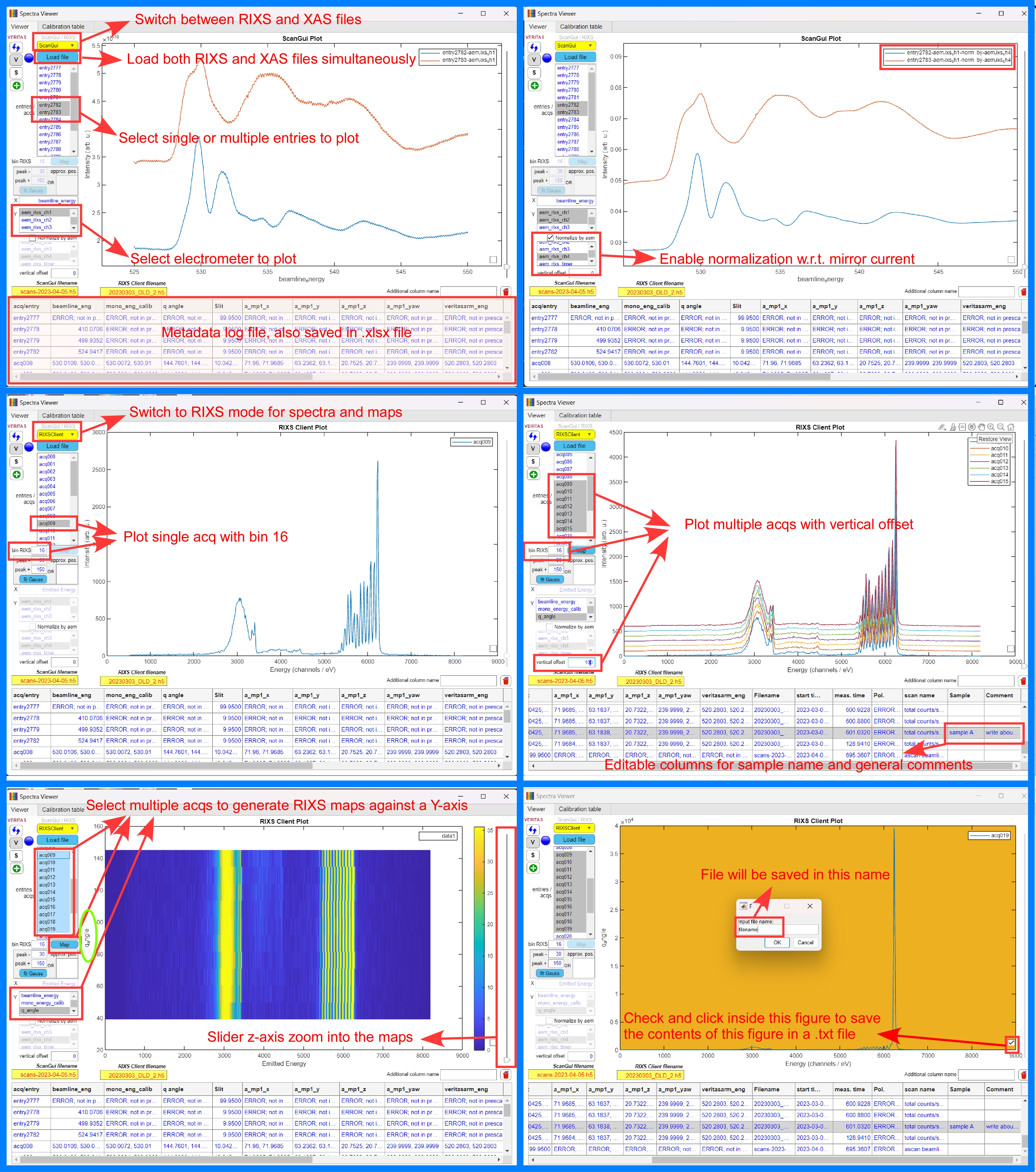
SpectraViewer interface with a few functionalities.
RIXS Analysis
Here you can do advanced analysis using the raw data from RIXS .h5 file. The figure shows the interface of the software. It has several tabs using which you can do different types of analysis, thereby utilizing the full potential of the Veritas beamline.
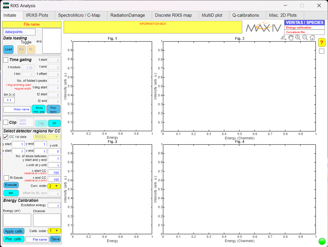
RIXS Analysis ineterface.
Here is a brief introduction to all these tabs and their functionalities:
Initiate –> start working with raw data. Apply the following filters: time gating, time gating background, start and end global time, mask out detector artifacts (is any), curvature correction (generate new or use the parameters from beamline), and energy callibration.
tRIXS Plots –> slice the spectrum in time from nano-seconds (bunch clock) to seconds (global clock), correct the energy drift in time (if any), plot continuous RIXS maps (without reconstructions of energy steps) and extract PFY from it.
Spectromicroscopy / C-map –> spatially scan the sample with 1X5 um^2 spatial resolution and extract the RIXS spectrum of individual 5 um^2 pixels. Understand the inhomogenity in electronic structure corresponding to a particular RIXS excitation feature. Also plots continuous RIXS maps.
RadiationDamage –> study the effect and evolution of radiation damage in samples. Selectively extracts RIXS spectra within the initial and end of exposure time at a particular spot. In this way you can do step resolved or step integarted beam damage analysis. Plots continuous RIXS maps with reconstruction of energy steps (more precise than the other two).
Discrete RIXS map –> plots RIXS maps from previously analysed files or the calibrated files available in the .h5 RIXS file. Extract PFY.
MultiD plot –> not available yet.
Q calibrations –> it allows you to calibrate the manipulator angles and estimate the relation among Q, scattering angles and manipulator angles.
Misc. 2D plots –> for testing.
You may download and install the latest version of RIXS Analysis software for Windows and MAC using the link
The figure shows an overview of all the tabs and salient functionalities.
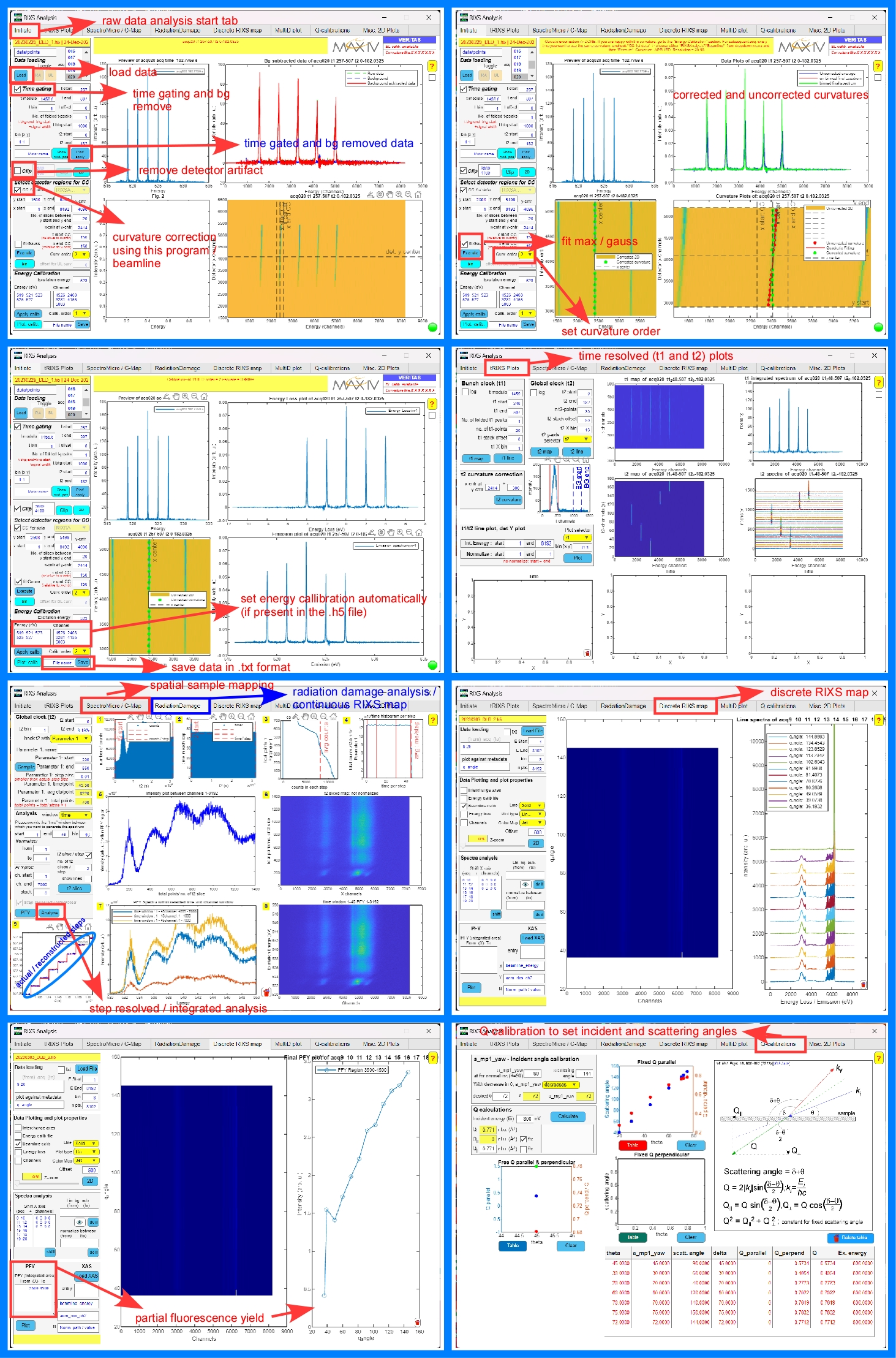
RIXS Analysis tabs and functionalities